Call Graph Construction Algorithms Explained
A call graph is an artifact produced by program analysis tools to record the relationships between a function and the functions it calls. If you’ve ever wondered how these call graphs actually get generated then keep reading because in this post I’ll be exploring several call graph construction algorithms and their tradeoffs.
Note: Some issues with the information in the RTA section of this article have been brought to my attention and will be fixed shortly. Thanks to David Bacon for pointing them out to me.
If you just want the nitty-gritty formal stuff then check out the paper by Tip and Palsberg, which inspired this post.
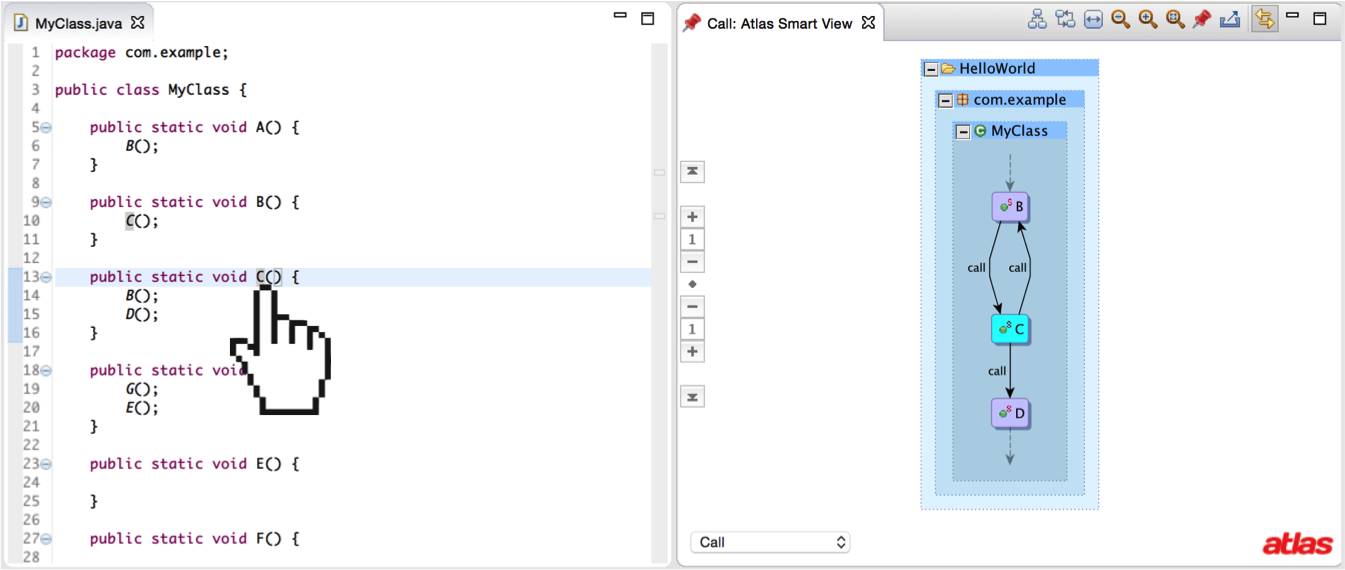
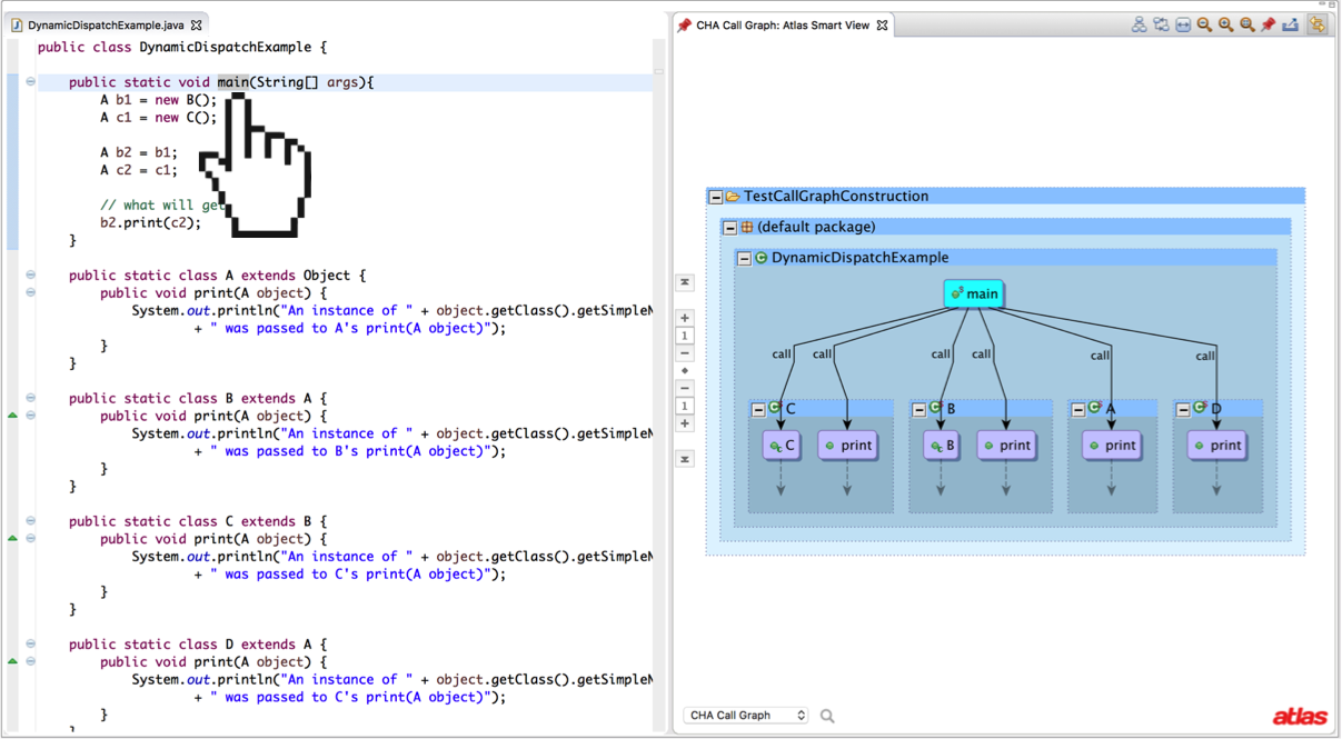
Let’s start by taking a look at a call graph. The figure below shows a call graph for a simple Java program that indicates the Java program has a method B that calls the method C and that C in turn calls methods B and D.
I’ve implemented each variation of the algorithms discussed in this post in an open source Eclipse plugin project called the call-graph-toolbox, which runs on top of the Atlas program analysis framework. Atlas provides an interface for creating Smart Views that allow you to click on source code or program graphs to instantly produce an updated program graph relevant to what you clicked. The call-graph-toolbox provides each call graph implementation as a Smart View so the differences in the algorithms can be observed visually. I’ll be using call-graph-toolbox to help show the differences of each algorithm discussed in this post.
The Problem(s)
Let’s start by understanding why it might be hard to create a call graph. To keep things simple we are just going to be considering Java, but know that the problem gets harder when we start talking about dynamically typed languages (such as Python or Ruby) or languages with function pointers (such as C, C++, or Objective-C).
Consider the following program.
- What will it print if we run it?
- What methods would be called at runtime?
- What edges should the ideal call graph have?
Static vs. Dynamic Dispatch
In Java, when we call a method, the binding between the callsite and the method to be called may be done at compile time or runtime. If the method binding is resolvable at compile time we call it a static dispatch. If at compile time we can’t resolve the callsite we call it a dynamic dispatch and resolve the callsite later at runtime. Dynamic dispatches are extremely common in Object Oriented languages like Java, so we should spend some time making sure we understand how they work.
Since a static dispatch is resolvable at compile time, we know exactly where to find the code for the method we are calling before we even run the program. In Java, calls to methods marked static and calls to constructors are both static dispatches. Since everything in Java is an object it makes sense that we should always know exactly where the code to construct new objects is located in our program. Methods that are marked static (class methods) do not require that we create an instance of an object to invoke the method. Every executable Java program has at least one static method, the main method, which makes sense because before we run the program we haven’t created any new objects yet, but we still want to invoke some procedure to use as an entry point into the program.
// a static dispatch can be called directly on a type without
// an instance such as this hypothetical class method that
// runs a simulation procedure
Animal.runSimulation();
Java methods that are not marked static (instance methods) require an instance of an object. We can imagine a Person class with a method getName() that returns the name of a person. Since we don’t want to assign the same name to all people, the getName() method should be associated with an instance of a person. This means we need to call getName() on a Person object (and not directly on the type like a class method). A call to an instance method is resolved at runtime using a dynamic dispatch and the reason why will become clear soon.
Let’s take a look at the print callsite in the main method of our example program from above. The print method is declared in class A and then overridden by A’s children in classes B, C, and D. We know that print is an instance method because it is not marked as a static method. If we run this program, the print method declared in class B will get executed. This is because the variable b2 is an object of type B. If you wanted to call the print method declared in class C you could replace b2 with c2. This means that we have to know the type of the object the instance method is being called on to know which method will get called at runtime!
Now remember that every object in Java can be drawn in a tree hierarchy with java.lang.Object at the very top. The type hierarchy for our small program is shown below.
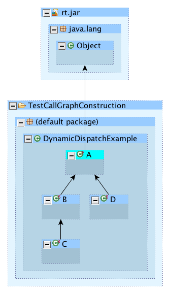
Any non-private instance method declared in a parent type is inherited by the child, unless that child provides an alternative implementation of the inherited method (by overriding the method). As a result of Java’s type hierarchy we can also assign any object type to a variable of the same type or a variable with the type of any of the object’s parent types (including java.lang.Object). This means that someone could write the following code.
Object o;

// getRandomObjectType() returns a declared type of
// java.lang.Object, which could be any runtime type
o = getRandomObjectType();

o.toString();
The instance method toString is declared in java.lang.Object so it can be called on any object type. Since we don’t know the type of the object in variable o we have to assume that java.lang.Object’s toString method or any object that overrides toString could be called at runtime! Since Java highly encourages developers to override the toString method this leaves us with quite a few possibilities (and only one correct answer).
To answer our questions from above, we would all probably agree that an edge from the print callsite (at b2.print(c2)) to B’s print method implementation should be in our call graph because B’s print method is what gets executed at runtime. We also know that it could be tricky to figure out exactly which method would get called at runtime as a result of a dynamic dispatch because it could be tricky to statically determine the runtime type of b2. So should we conservatively add edges to A, B, C, and D’s print methods if we can’t figure out the type of b2 even though A, C, and D’s print methods are never called? What’s better a call graph with all of the possible edges or a call graph with only the edges we are sure are correct?
We say a call graph is “sound” if it has all the edges that are possible at runtime. We say a call graph is “precise” if it does not have edges that do not occur at runtime. It’s easy to be sound, but its hard to be sound and precise.
Whole vs. Partial Program Analysis
Partial program analysis occurs when we don’t have the entire program or when we can’t scale up our analysis to run over the entire program. You might think your Hello World program is small, but don’t forget you are running it on top of a vast set of libraries provided with the Java Runtime Environment. If you’re really crazy you might also consider the native implementation of the virtual machine itself or the operating system that virtual machine is running on and so on and so on!
In practice sometimes we just want to analyze a specific library, which could be used by many applications, so we are forced to do partial program analysis. Consider our example from before. What would happen if we removed the main method and just consider the classes A, B, C, and D? Since the main method is the only place any types are actually created, it would look like the four print instance methods are just dead code, but don’t forget that this “library” could be used by any Java program! Since we could conceive of Java programs that could call all four print methods we can’t consider any of them dead code. So with that in mind it is going to be important to specify whether or not we are analyzing a partial program or a whole program when we construct our call graphs.
Idea 1 - Class Hierarchy Analysis (CHA)
Let’s start by building a sound call graph (we’ll worry about precision later). The first algorithm you might think to implement would probably be a variation of Reachability Analysis (RA). The basic idea is that for each method, we visit each callsite and then get the name of the method the callsite is referencing. We then add an edge from the method containing the callsite to every method with the same name as the callsite.
REACHABILITY ANALYSIS
for each method (M)
   for each callsite (C) in M
       if C is a static dispatch
          add an edge to the statically resolved method
       otherwise,
          M' = methods with the same name as the callsite C
          create edge M -> M'
The result is a completely sound call graph, but not a very precise call graph. We might even match callsites of print(Object o) to a method that takes a different number of parameters such as print(Object o1, Object o2). We could make our matching implementation stronger by matching the entire method signature (method name, method parameter counts/types, return type), but we still are going to have plenty of bad (conservative) matches. Consider the following code snippet with respect to our first example.
B b = new B();

// ...some stuff happens

// dispatch goes to B's print or at least
// a child of B that overrides B's print
b.print(b);
A simple reachability analysis would add edges from the print callsite to A, B, C, and D’s print methods, but we declared b as a B type so we know the dispatch has to at least go to B or a child of B’s print method. We don’t know what happened in the ..., so it is possible that an instance of a C type could have been assigned to b.
B b = new B();
b = new C(); // dispatch now goes to C's print
b.print(b);
At this point it should be becoming clear that we could improve upon RA by considering the type hierarchy. Class Hierarchy Analysis (CHA) was first proposed in a 1995 paper by Dean, Grove, and Chambers to do just this. Class Hierarchy Analysis looks at the declared type of the variable (the receiver object) used to invoke the dynamic dispatch and restricts call edges to the inherited method implementation or the methods declared in the subtype hierarchy of the declared type of the receiver object. The result is a vast improvement on RA that is still sound and cheap to compute.
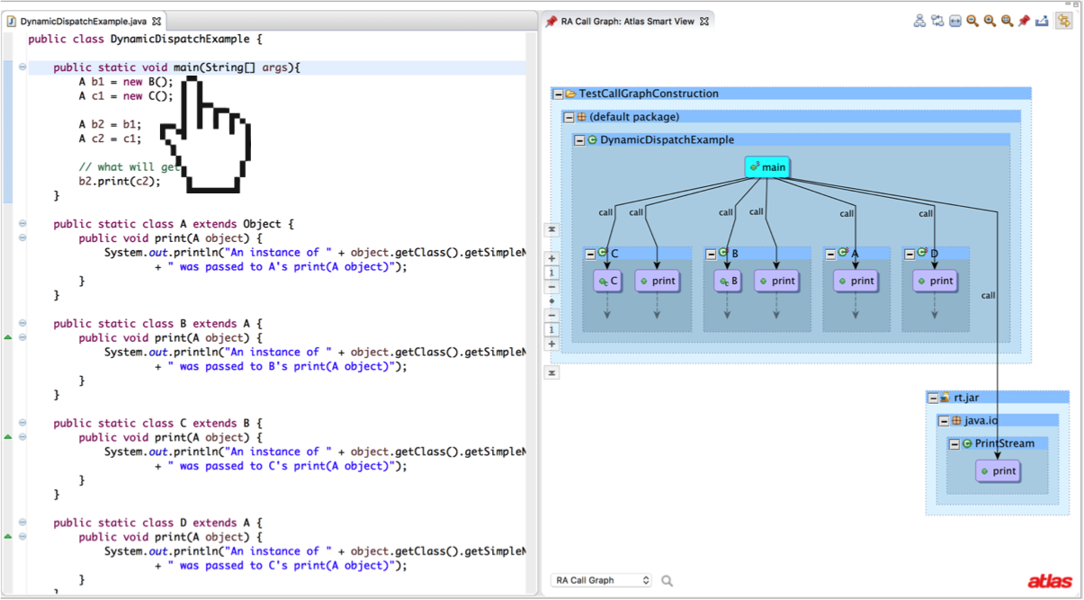
I’ve implemented both RA and CHA call graph construction algorithms in my call-graph-toolbox. The results for our first example are shown below. Note that RA picks up an extra print method signature in java.io.PrintStream.
Now let’s take a look at how CHA would do when analyzing a library. For the most part, it does pretty well! A class hierarchy analysis doesn’t care about where the types are instantiated, since it only uses the declared type of the receiver object. The only tricky part is that an application could declare a type that overrides an instance method in the library, in which case the dynamic dispatch could actually dispatch to a method outside of the library (an application callback). So how can we create a call edge for a method that doesn’t exist yet!? Well all we have to work with is the fact that whatever method is going to override our library method has to be in a subtype of the library’s type that declared the method being overridden.
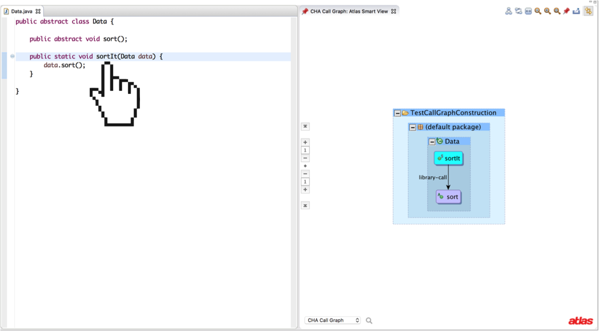
Consider the case where a library defines a single abstract class with a method sort. The library contains no subtypes of Data that implement the sort method. Somewhere else in the library a call to the sort method is made. At runtime a subtype of Data will exist with a sort method, but not when the library was compiled. The best place I’ve seen this problem defined is as the Separate Compilation Assumption by Karim Ali.
public abstract class Data {

   public abstract void sort();

   public static void sortIt(Data data) {
      data.sort();
   }
}
There is no concrete method implementation for sort in our library, so adding a call edge from sortIt to sort might be a bit misleading (because Data’s sort method can’t actually be a runtime dispatch target). Instead what we could do is modify CHA to add a “library-call” edge to sort to indicate that any dynamic dispatch that gets resolved at runtime must override sort. Running the call-graph-toolbox algorithm for CHA in library mode (available in the Eclipse preference menu) for this example shows an example of a “library-call” edge. Aside from abstract methods without any concrete method implementations, remember that any non-final method in any non-final class could be overridden by an application to form a callback.
Idea 2 - Rapid Type Analysis (RTA)
Class Hierarchy Analysis gives us a sound and cheap call graph. In fact it is the default call graph implementation for most static analysis tools (including Atlas), but can we do better? Remember that a dynamic dispatch has to be called on an instance of an object, which means that in order for a dispatch to be made to a particular type’s instance method at least one object of that type (or subtype) must have been allocated somewhere in the program. This is the core idea behind Rapid Type Analysis (RTA), which was proposed by Bacon and Sweeney (implementation details available in the extended technical report).
Object o1 = new A(); // new allocation of type A!
Object o2 = new B(); // new allocation of type B!
Object o3;

// ... some stuff happens

// If only A and B types were allocated, then its a good
// guess that o3 is either an A or B type too
o3.toString();
Given a CHA call graph we start at the main method and iteratively construct a new call graph that is a subset of the CHA call graph by adding only the edges to the methods that are contained in types of objects that were allocated in the main method. The methods that are reachable through the newly added edges are added to a worklist and the process is repeated until the worklist is empty.
Methods can be inherited from parent types so we should consider the supertypes of the allocated types as well. RTA considers that a type could be allocated in a method and then passed as a parameter to another method. Since the resolved calling relationships are being built on-the-fly it’s important to note that RTA may evaluate a method several times (if new callers are discovered the method has to be re-evaluated). RTA runs until the worklist is empty, at which point it has reached a fixed point and cannot resolve any new call edges to add to the call graph.
RAPID TYPE ANALYSIS
RTA = call graph of only methods (no edges)
CHA = class hierarchy analysis call graph
W = worklist containing the main method
while W is not empty
   M = next method in W
   T = set of allocated types in M
   T = T union allocated types in RTA callers of M
   for each callsite (C) in M
     if C is a static dispatch
        add an edge to the statically resolved method
     otherwise,
        M' = methods called from M in CHA
        M' = M' intersection methods declared in T or supertypes of T
        add an edge from the method M to each method in M'
        add each method in M' to W
The result of RTA on our first example is shown below.
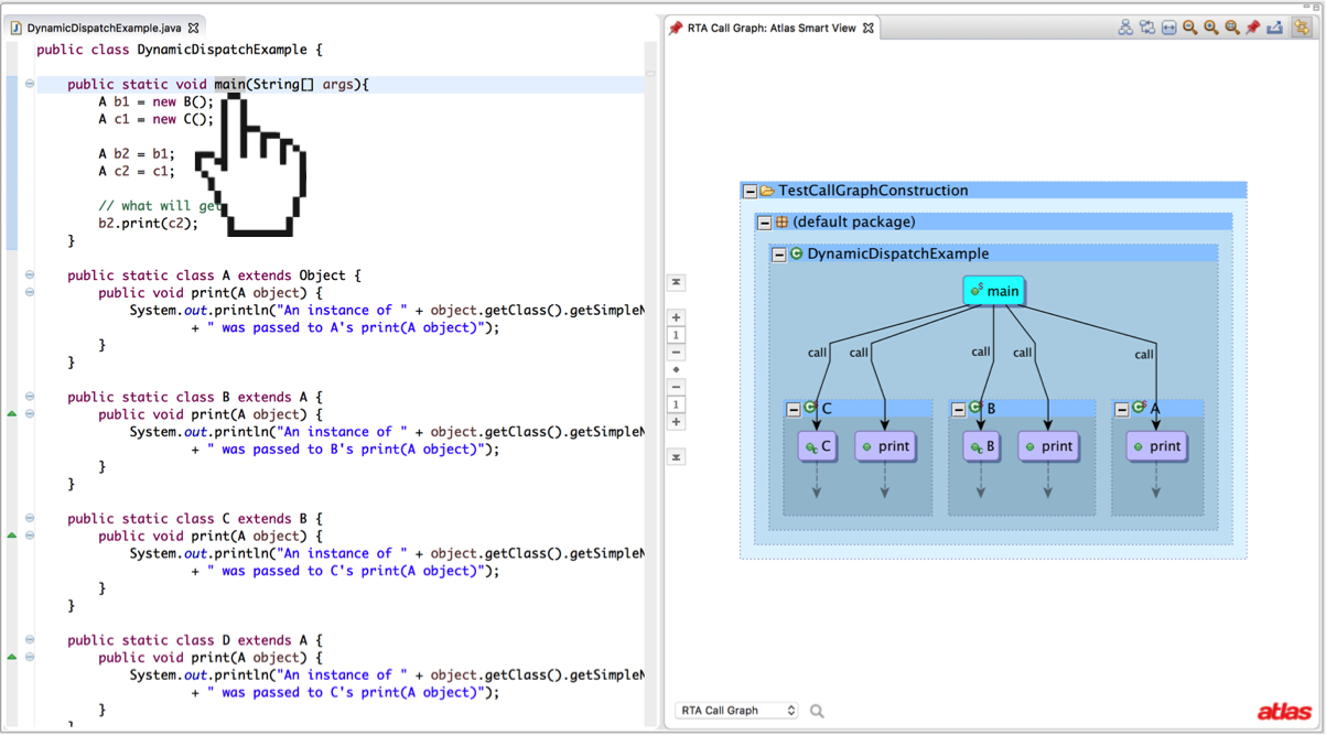
RTA produces a more precise call graph than CHA (because it is a subset of CHA and removes edges that are likely not feasible at runtime), but the result is no longer sound. Let’s consider a few cases where RTA might not produce a sound call graph.
public static Object v;

public static void main(String[] args){
   foo();
   bar();
}

public static void foo(){
   Object o = new A();
   v = o;
}

public static void bar(){
   v.toString()
}
In the example above main calls foo, which allocates a new A type and stores the instance to a field v. Then main calls bar, which accesses the field and calls toString on the instance stored in v. RTA will not include an edge from bar to toString because neither bar or its parents (main) allocated any instance that toString could be called on (however some implementations might consider the String[] args to be a special implicit allocation of an array type of String types, but the type A still does not reach bar in the basic RTA implementation).
Let’s consider another example of unsoundness.
public static void main(String[] args){
   Object o = foo();
   bar(o);
}

public static Object foo(){
   return new A();
}

public static void bar(Object o){
   o.toString()
}
In this example main calls foo, which returns an allocation of type A that is then passed as a parameter in the call to bar. Again in this case the call edge to A’s toString method would be missing because neither bar or its parents (main) allocated a type of A.
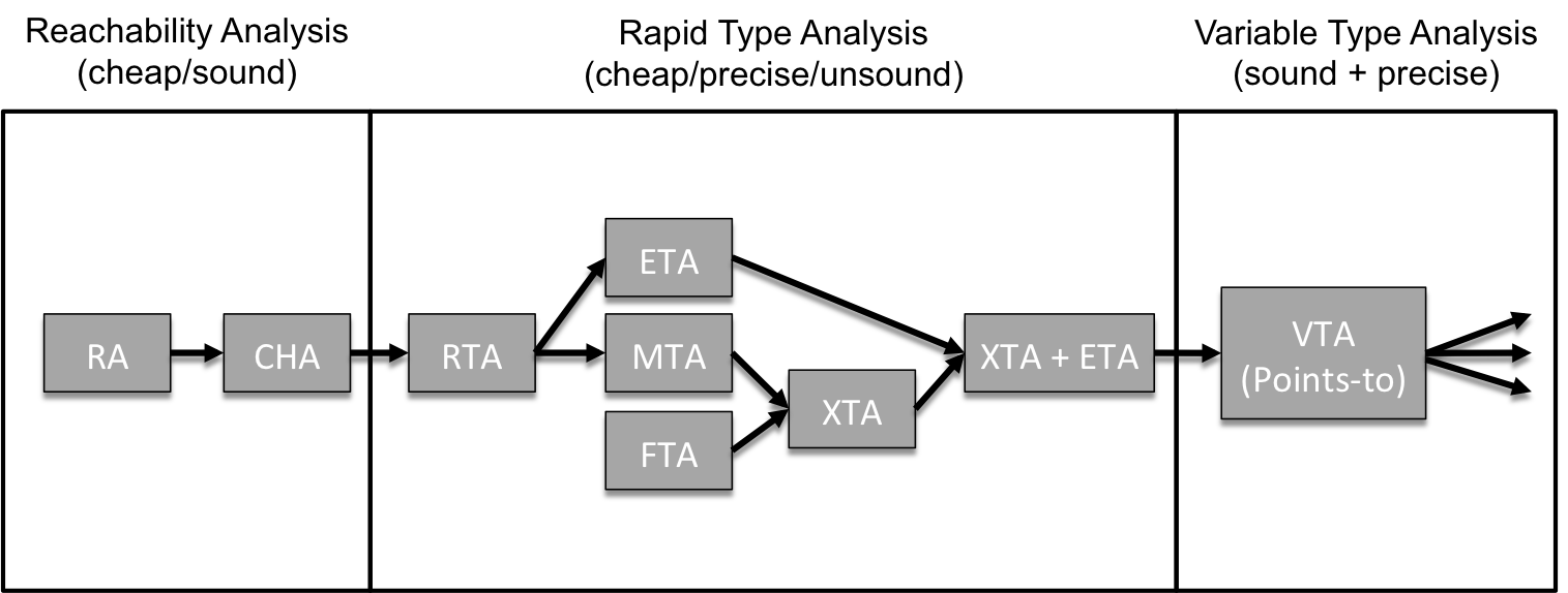
As you may have guessed we could modify RTA to consider fields and the types of method parameters and method return types to improve the accuracy of RTA, which is exactly what Tip and Palsberg proposed to do in the paper that inspired this post. In their paper, Tip and Palsberg propose to add several more constraints to RTA.
The first set of constraints concerns global variables and forms the basis for the first variation of RTA, Field Type Analysis (FTA). FTA adds the constraint that any method that reads from a field can inherit the field-compatible allocated types of any method that could write to that field.
The second variation of RTA, Method Type Analysis (MTA), adds constraints involving method parameter types and method return types. MTA adds the constraint that types allocated in a method and then passed to a method through a parameter should be compatible with the called method’s parameter types. MTA also adds the constraint that the return type of each called method be added to the set of allocated types. At first this may seem difficult because the return type would appear to depend on the resolution of dynamic dispatches, but the set of potential dynamic dispatches are statically typed to be the same return type.
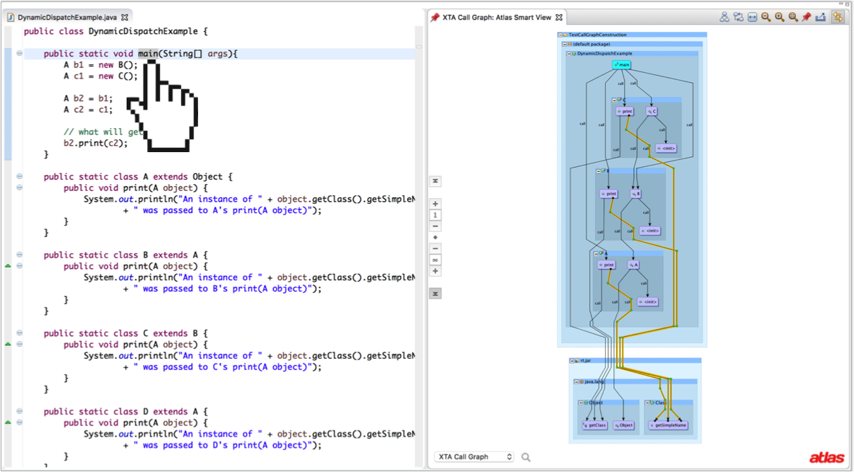
Finally, we can combine both sets of constraints defined by MTA and FTA to form a Hybrid Type Analysis (XTA). The result of XTA on our first example is shown below. Note that the call graph depth has been expanded to reveal three newly resolved dispatches to getSimpleName, which are not resolved by RTA because the instance of the Class object is returned by getClass.
The idea of adding constraints to RTA to improve the accuracy and soundness of the base algorithm is an interesting idea and worth pursuing deeper. If we assume the standard Von Neumann model of a computer, then programs can only communicate data through the stack or the heap. FTA adds constraints for communicating through the heap when new allocations are created and stored in a global variable, while MTA adds additional constraints for communicating through the stack when methods are called with parameters and then subsequently return results. One other way to pass information is by creating and throwing an exception. Tip and Palsberg mention exception handling as an implementation issue, but do not propose a set of contraints to use as an approximation for analyzing programs with exceptions.
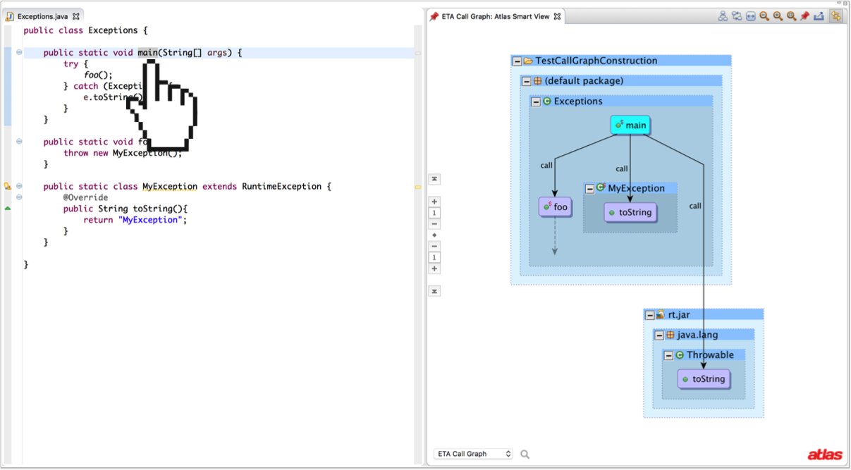
Since exception handling is extremely common in Java code, I propose another RTA variation, Exception Type Analysis (ETA), which adds the following constraint. Add the allocated and inherited types of any method with a throw site to every method that contains a reachable type compatible catch block in the current reverse call graph of throwing method. Of course this constraint could be added to XTA, so we should differentiate between the classic XTA and XTA with ETA. The result of ETA for the following code snippet is shown below.
public class Exceptions {

   public static void main(String[] args) {
      try {
         foo();
      } catch (Exception e){
         e.toString();
      }
   }

   public static void foo() {
      throw new MyException();
   }

   public static class MyException extends RuntimeException {
      @Override
      public String toString(){
         return "MyException";
      }
   }
}
Note that none of the RTA variants proposed by Tip and Palsberg specifically address this case and would fail to add the edge to MyException’s toString method.
Now let’s play out the idea of adding constraints a bit further. Consider how RTA would address the following snippet of code.
Object o1 = new A();
Object o2 = new B();
o2.toString();
The variable o1 is assigned an allocation of type A and then the variable o2 is assigned an allocation of type B. RTA is only looking at the allocation types, so the fact that o2 could only be a type B is lost in the approximation. Without considering the assignments that were made to the variable o2 it is impossible to rule out any other dispatch possibilities. We are reaching the point where we can no longer add any more constraints to refine the precision of our call graph without trying to directly determine the type of the variable for the callsite, which brings us to Variable Type Analysis (VTA) in the next section.
Before we move on, let’s consider how RTA performs on a library. Since RTA starts with a worklist containing only the main method, a library without a main method would result in an empty call graph without some modifications to RTA. Without the application code that is using the library, we have to assume that any method could be called by the application. Depending on how many assumptions we want to make we could restrict that set to say only public methods in the library, but we’d be ruling out the fact that an application might extend a type and inherit a protected method or use reflection to call a private method.
We should also assume that the application could allocate any type and pass it to a method, which pretty much brings us back to a Class Hierarchy Analysis in terms of precision. FTA and MTA would fair better than RTA alone for this last assumption as they would at least filter those types based on the compatibility of their types. Finally there is still the possibility the library contains calls to abstract methods that do not have any concrete implementations, so RTA should at least include the library calls calculated in CHA.
Idea 3 - Variable Type Analysis (VTA)
The last approach is rather direct. We have a reference to the variable that is used in the callsite, but we need to learn know its type. One rather straightforward idea is to start at every allocation site and record its type. Then we iterate over every assignment building a graph of each variable and the assignment of the allocation type to a variable or an assignment of a variable to a variable. At the end we can use the graph to answer which set of types a variable could point to based on what could have been assigned to that variable during the execution of the program.
The algorithm looks remarkably similar to RTA in that it is a fixed point algorithm using a worklist, but since we are considering much more information than RTA the cost of running VTA is going to be much higher. Without getting too deep into points-to analysis (a subject for another day) it’d be good to note that a VTA implementation could be accomplished with an implementation of a full blown points-to, which tracks the allocation site that each variable in the program could point-to, or a slimmed down version of a points-to that is only tracking the type of the allocation site for each variable in the program.
The precision of VTA is going to be much better than RTA, but depends on a whole new set of hard problems in computer science that is the focus of much of the recent research in this area. I’ll group all of these problems into one bucket and call them “sensitivities”. One such sensitivity is “flow sensitivity”, which refers to whether or not the ordering of the assignments is taken into account. For example if we assigned the result of a new A type allocation to a variable o and then immediately overwrote the value of o with a different allocation type of B, a locally flow-sensitive implementation could take advantage of the fact that o could only be of type B immediately after the second assignment.
Object o = new A();
o = new B();
o.toString();
For basic blocks it’s possible to be locally flow-sensitive relatively easily using a Static Single Assignment (SSA) form, but things get tricky when we start talking about loops or the ordering of inter-procedural flows (also known as context-sensitivity). In fact, we know a perfectly precise points-to analysis is simply not possible, because the entire problem can be reduced to the halting problem (see Landi, Ramalingam, Reps).
The call graph toolbox implements a call graph based on the results of a context-insensitive points-to analysis I wrote available in the points-to toolbox. A context-insensitive points-to analysis is called a 0-CFA (when context is defined as calling context). The results for our first example are shown below.
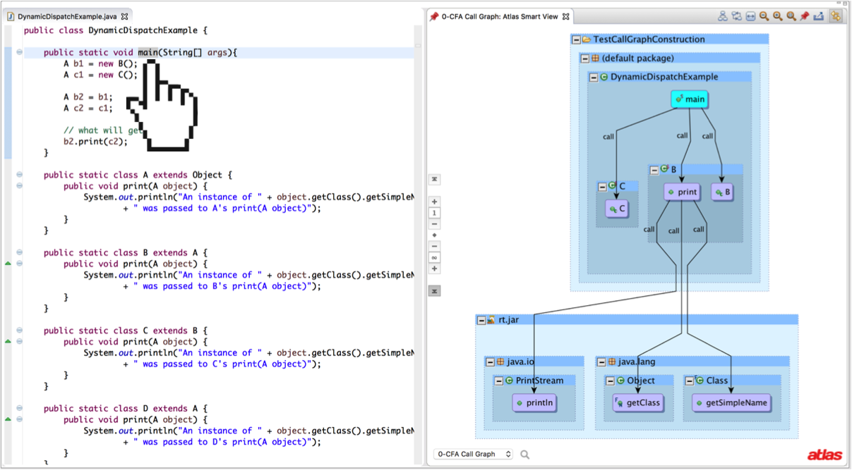
In general a points-to based call graph will suffer from similar ailments as RTA and its variants when it comes to library analysis. The difficultly in being precise is not knowing what could happen outside of the code being analyzed. Without a main method a points-to analysis has to consider every allocation type as being possible at runtime and propagate that information forward until a fixed point is reached, but this can be incredibly expensive for large applications. Current research focuses on performing precise yet scalable points-to analysis because it is the basis for solving many program analysis tasks (such as alias analysis, type inference, and call graph construction).
Evaluation and Conclusion
So…which call graph construction algorithm should I use? Well let’s run some numbers on a large application and see.
ConnectBot (Android Application)
Personally, when I test out a new program analysis tool, I like to use the Android application ConnectBot because I’m familiar with it, it is open source, it is fairly large (~235 classes, 33K logical lines of code), and it is decently complex. The developer(s) always seem to do something a little differently than you would expect.
For instance, ConnectBot has an abstract class that defines a concrete method, which is then intentionally overridden by all the abstract class’s children. The base method is an empty method implementation that just has a comment to the effect of “all base classes should override this method”, which just pains me to see because without marking the method abstract we can’t actually guarantee that all children will implement the method. It’s a bug waiting to happen if a new developer doesn’t notice this pattern and accidently, but silently inherits the empty implementation from its parent type. This is one of the reasons why we have abstract methods in the first place!
So if it is true that all the children override the concrete method and the base method’s type cannot be instantiated (because it’s abstract) then the base method is actually dead code and should be removed from the CHA result. Thank you ConnectBot developers for making my program analysis code better by writing goofy code, but…
The results of running each call graph construction algorithm on ConnectBot are shown in the table below.
ConnectBot contains 9,966 callsites with 3,938 static dispatches and 6,028 dynamic dispatches. Of the 6,028 dynamic dispatch callsites, I computed the minimum, maximum, and average number of potential dispatch targets each algorithm resolved. The number of nodes refers to the number of methods in the resulting call graph, whereas the number of edges refers to the number of call edge relationships in the resulting call graph.
It’s also important to note that ConnectBot is an Android application, which means it does not have a main method. It is possible to model the Android lifecycle to figure out the application entry points, but that was not done for this analysis and the call graphs were simply produced using the library assumptions stated earlier for each algorithm.
| Algorithm | Time (Seconds) | Nodes | Edges | Min | Max | Average |
|---|---|---|---|---|---|---|
| RA | 452.96 | 4,065 | 30,067 | 1 | 91 | 6.25 |
| CHA | 75.38 | 3,490 | 9,400 | 1 | 31 | 1.40 |
| RTA | 29.03 | 2,515 | 5,166 | 0 | 5 | 0.50 |
| FTA | 128.12 | 2,963 | 6,969 | 0 | 12 | 0.93 |
| MTA | 38.04 | 2,629 | 5,462 | 0 | 5 | 0.58 |
| ETA | 177.02 | 2,503 | 5,359 | 0 | 11 | 0.52 |
| XTA | 94.52 | 2,987 | 6,776 | 0 | 10 | 0.81 |
| XTA + ETA | 279.82 | 2,954 | 6,860 | 0 | 15 | 0.83 |
| 0-CFA (Points-to) | 37.51 | 3,073 | 6,388 | 0 | 9 | 1.09 |
The time column should be taken with a grain of salt. I implemented most algorithms focusing on correctness and readability and didn’t optimize the code too heavily (some caching would go a long way). The points-to analysis on the hand is very optimized code and completes in under half a second and the results are then used to reconstruct the call and control flow graphs after the fact.
Aside from timing, the Min column is interesting. In this table we are including library calls (call edges to abstract methods when no implementation is available) so a callsite with no resolvable dispatches means the algorithm is unsound. We should expect this from RTA and its variants and depending on the implementation, points-to analysis as well. In this case, the points-to analysis is unsound because it was not considering new allocations that occur inside the Java Runtime libraries.
The Average column is also interesting. At runtime only one dispatch target is actually possible for a callsite at a given point in the program execution (its possible the callsite location could be a different target at a later point in the execution). So in an ideal world, our static analysis tool would report exactly one potential dispatch target for each callsite (in a given context). An average number of potential dispatch targets that approaches 1.0 is a sign of a precise call graph. In our results the 0-CFA is the closest to the ideal value.
Apache Commons IO (Application Mode)
Let’s analyze one more application just so we can try out whole program analysis. For this project, I downloaded the source code of the Apache Commons IO 2.4 library and imported all library code into an Eclipse project. I then included the HexDumpTest test from the test package. To make things simple I remove the JUnit assertions and added a main method that created a new HexDumpTest and called the testDump. The results are shown in the table below.
The project contained 2,931 callsites, with 1,634 static dispatches and 1,297 dynamic dispatches.
| Algorithm | Time (Seconds) | Nodes | Edges | Min | Max | Average |
|---|---|---|---|---|---|---|
| RA | 42.64 | 2,005 | 12,700 | 0 | 80 | 11.03 |
| CHA | 6.95 | 1,817 | 5,119 | 0 | 80 | 3.26 |
| RTA | 0.07 | 31 | 34 | 0 | 3 | 0.02 |
| FTA | 0.19 | 45 | 51 | 0 | 3 | 0.02 |
| MTA | 0.1 | 30 | 33 | 0 | 3 | 0.02 |
| ETA | 0.18 | 31 | 34 | 0 | 3 | 0.02 |
| XTA | 0.28 | 50 | 58 | 0 | 3 | 0.02 |
| XTA + ETA | 0.53 | 51 | 60 | 0 | 3 | 0.04 |
| 0-CFA (Points-to) | 2.3 | 1,325 | 2,126 | 0 | 8 | 0.85 |
In this table the Min, Max, and Average columns should be taken with another grain of salt because we are only considering methods reachable from the main method, so callsites outside of that reachable set of methods are dead code and should not have resolvable targets!
Apache Commons IO (Library Mode)
For comparison, I commented out the HexDumpTest.main method and collected the table statistics again with library analysis enabled. Without the main method, the project contained 2,929 callsites, with 1,633 static dispatches and 1,296 dynamic dispatches.
| Algorithm | Time (Seconds) | Nodes | Edges | Min | Max | Average |
|---|---|---|---|---|---|---|
| RA | 43.94 | 2,139 | 13,874 | 1 | 83 | 12.21 |
| CHA | 7.25 | 1,882 | 5,298 | 1 | 80 | 3.42 |
| RTA | 5.12 | 1,159 | 1,812 | 0 | 10 | 0.59 |
| FTA | 10.11 | 1,280 | 2,201 | 0 | 15 | 0.91 |
| MTA | 6.84 | 1,196 | 1,837 | 0 | 4 | 0.63 |
| ETA | 9.28 | 1,154 | 1,784 | 0 | 8 | 0.56 |
| XTA | 10.81 | 1,321 | 2,138 | 0 | 9 | 0.89 |
| XTA + ETA | 14.54 | 1,321 | 2,152 | 0 | 10 | 0.91 |
| 0-CFA (Points-to) | 2.39 | 1,400 | 2,303 | 0 | 9 | 1.01 |
So to answer the question, which algorithm is the best? CHA is a great contender for when soundness is required and we don’t want to invest a lot of computation time. If we can relax the soundness requirement a bit we might consider RTA or one of its variants, but in my experience most research is trending towards figuring out how to scale a points-to analysis for sound-ish and precise results.
Closing Thoughts
Tip and Palsberg present a nice overview diagram in Figure 1 of their paper, which I have reproduced below with some modifications.